Posts filed under Probability (66)

November 17, 2017

Lotto

Q: Can I improve my chances of winning Lotto by…

A: No.

Q: But….

A: No.

Q: …

A: Just no.

Q: … by buying a ticket?

A: Ok, yes. But not by very much.

Q: You sound like you’ve been asked about Lotto odds a lot.

A: There’s a larger-than-usual jackpot in the NZ Powerball

Q: Enough to make it worth buying a ticket?

A: If you like playing lotto, sure.

Q: No, as an investment.

A: I refer the honourable gentleman to the answer given some moments ago

Q: Huh?

A: No.

Q: But $35 million. And a 1 in 38 million chance of winning. And 80c tickets.  Buying all the tickets would cost less than $30 million. So, positive expected return.

A: If you were the only person playing

Q: And if I’m not?

A: Then you might have to share the prize

Q: How many other people will be playing?

A: Lotto NZ says they expect to sell more than a million tickets

Q: Compared to 38 million possibilities that doesn’t sound much

A: That’s tickets. Not lines.

Q: Ah. How many lines?

A: They don’t say.

Q: Couldn’t the media report that instead of bogus claims about a chemist in Hawkes Bay selling better tickets?

A: Probably not. I don’t think Lotto NZ tells them.

Q: That story says it would take 900 years to earn the money at minimum wage. How long to get it by playing Powerball?

A: At, say, ten lines twice per week?

Q: Sure.

A: 36900 years.

June 13, 2016

Reasonable grounds

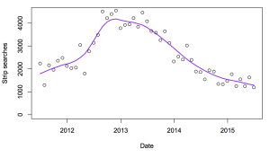
Mark Hanna submitted an OIA request about strip searches in NZ prisons, which carried out with ‘reasonable grounds to believe’ the prisoner has an unauthorised item.  You can see the full response at FYI. He commented that 99.3% of these searches find nothing.

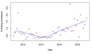
Here’s the monthly data over time:

searches
The positive predictive value of having ‘reasonable grounds’  is increasing, and is up to about 1.5% now. That’s still pretty low. How ‘reasonable’ it is depends on what proportion of the time people who aren’t searched have unauthorised items: if that were, say, 1 in 1000, having ‘reasonable grounds’ would be increasing it 5-15-fold, which might conceivably count as reasonable.

We can look at the number of searches conducted, to see if that tells us anything about trends
conducted
Again, there’s a little good news: the number of strip searches has fallen over the the past couple of years. That’s a real rise and fall — the prison population has been much more stable. The trend looks very much like the first trend upside down.

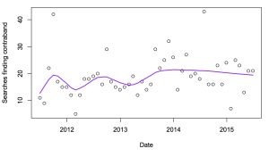
Here’s the trend for number (not proportion) of searches finding something
finds
It’s pretty much constant over time.

Statistical models confirm what the pictures suggest: the number of successful searches is essentially uncorrelated with the total number of searches. This is also basically good news (for the future, if not the past): it suggests that a further reduction in strip searches may well be possible at no extra risk.

May 4, 2016

Should you have bet on Leicester City?

As you know, Leicester City won the English Premier League this week. At the start of the season, you could get 5000:1 odds on this happening. Twelve people did.

Now, most weeks someone wins NZ Lotto first division, which pays more than 5000:1 for a winning ticket, and where we know the odds are actually unfavourable to the punter. The 5000:1 odds on their own aren’t enough to conclude the bookies had it wrong.  Lotto is different because we have good reasons to know that the probabilities are very small, based on how the numbers are drawn. With soccer, we’re relying on much weaker evidence.

Here’s Tim Gowers explaining why 5000:1 should have been obviously too extreme

The argument that we know how things work from following the game for years or even decades is convincing if all you want to prove is that it is very unlikely that a team like Leicester will win. But here we want to prove that the odds are not just low, but one-in-five-thousand low.

Professor Gowers does leave half the question unexamined, though

I’m ignoring here the well-known question of whether it is sensible to take unlikely bets just because your expected gain is positive. I’m just wondering whether the expected gain was positive.


March 29, 2016

Chocolate probabilities

For those of you from other parts of the world, there has been a small sensation over the weekend here about Cadburys chocolate randomisation. One of their products was a large chocolate egg accompanied by eight miniature chocolate bars, chosen randomly from five varieties.  Public opinion on the desirability of some of these varieties is more polarised that for others.

Stuff reports:

But one family found seven Cherry Ripes out of eight bars and most of those complaining to Cadbury say they found at least six Cherry Ripes out of eight. 

Cadbury claimed that it was just bad luck saying the chocolates are processed randomly and the Cherry Ripe overdose was not intentional. 

Both Stuff and The Guardian got advice on the probabilities. They get different answers: Martin Hazelton says seven out of eight being the same (of any variety) is about 1 in 10,000 and the Guardian’s two advisers say there’s nearly a 1 in 100 chance of getting seven Cherry Ripes out of eight (which is obviously less likely than getting seven of eight the same).

With a hundred-fold difference in the estimates, I think a tie-breaker is in order. Also, I’m going to do this the modern way: by simulation rather than by being clever. It’s much more reliable.

I’m going to trust the Guardian on what the five flavours were (since it doesn’t actually matter, I think this is safe).  I’ve put the code and results for 100,000 simulated packages up here.  The number of packs with seven or more bars the same was 44 out of 100,000. There’s obviously some random uncertainty here, but a 95% confidence interval for the proportion goes from 3 in 10,000 to 6 in 10,000, and so excludes both of the published estimates .  Since computing time is nearly free, and the previous run took only 13 seconds, I tried it on a million simulated packs just to be sure, and also separated out ‘seven or more of anything’ from ‘seven or more Cherry Ripes’.

Out of a million simulated packs, 442 had seven or more of some type of bar, and 83 had seven or more Cherry Ripes.  The probability of seven or more of something is between 4 and 5 out of 10,000 and the probability of seven or more Cherry Ripes is between 0.6 and 1 out of 10,000. It looks as though Professor Hazelton’s estimate of ‘a little less than one in 10,000‘ is correct for Cherry Ripes specifically.  The Guardian figures seem clearly wrong. The Guardian is also wrong about the probability of getting at least one of each type, which this code shows to be about 30%, not the 7% they give.

I said I wasn’t going to do this by maths, but now I know the answer I’m going to go out on a limb here and guess that Martin Hazelton’s probability was, in maths terms, P(Binom(8, o.2)≥7), which is the answer I would have given for Cherry Ripes specifically. With Jack and Andrew in the Guardian I think the issue is that they have counted all 495 possible aggregate outcomes as being equally likely, when it’s actually the 32768 390625 underlying ordered outcomes that are equally likely.

The other aspect of this computation is the alternative hypothesis. It makes no sense that Cadbury would just load up the bags with Cherry Ripes and pretend they hadn’t — especially as the Guardian reports other sorts of complaints as well. We need to ask not just whether the reports would be surprising if the bags were randomised, but whether there’s another explanation that fits the data better.

The Guardian story hints at a possibility: clumping together of similar chocolates. It also would be conceivable that the randomisation wasn’t quite even — that, say,  Cherry Ripes were 25% instead of the intended 20%. It’s easy to modify the code for unequal probabilities. Having one chocolate type at 25% doubles the number of seven-or-more coincidences, and more than half of them are now with Cherry Ripes. But that’s quite a big imbalance to go unnoticed at Cadburys, and it doesn’t push the probability a lot.

So, I’d say bad luck is a feasible explanation, but it could easily have been aggravated by imperfect randomisation at Cadburys.

Many lessons could be drawn from this story: that simulation is a good way to do slightly complicated probability questions; that people see departures from randomness far too easily; that Cadburys should have done systematic sampling rather than random sampling; maybe even that innovative maths teachers may have gone too far in rejecting contrived ball-out-of-urn problems as having no Real World use.

March 11, 2016

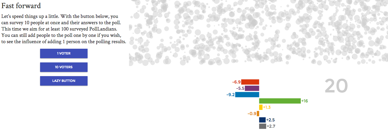
Getting to see opinion poll uncertainty

Rock’n Poll has a lovely guide to sampling uncertainty in election polls, guiding you step by step to see how approximate the results would be in the best of all possible worlds. Highly recommended.

Of course, we’re not in the best of all possible worlds, and in addition to pure sampling uncertainty we have ‘house effects’ due to different methodology between polling firms and ‘design effects’ due to the way the surveys compensate for non-response.  And on top of that there are problems with the hypothetical question ‘if an election were held tomorrow’, and probably issues with people not wanting to be honest.

Even so, the basic sampling uncertainty gives a good guide to the error in opinion polls, and anything that makes it easier to understand is worth having.

poll-land

(via Harkanwal Singh)

February 28, 2016

Forecasts and betting

The StatsChat rugby predictions are pretty good, but not different enough from general educated opinion that you could make serious money betting with them.

By contrast, there’s a professor of political science who has an election forecasting model with a 97+% chance that Trump will be president if he is the Republican nominee.

If you were in the UK or NZ, and you actually believed this predicted probability, you could go to PaddyPower.com and bet at 9/4 on Trump winning  and at 3/1 on Rubio being the nominee. If you bet $3x on Trump and hedge with $1x on Rubio, you’ll almost certainly get your money back if Trump isn’t the nominee, and the prediction says you’ll have a 97% chance of more than doubling your money if he is.

Since I’m not betting like that, you can deduce I think the 97% chance is wildly inflated.

February 13, 2016

Just one more…

NPR’s Planet Money ran an interesting podcast in mid-January of this year. I recommend you take the time to listen to it.

The show discussed the idea that there are problems in the way that we do science — in this case that our continual reliance on hypothesis testing (or statistical significance) is leading to many scientifically spurious results. As a Bayesian, that comes as no surprise. One section of the show, however, piqued my pedagogical curiosity:

STEVE LINDSAY: OK. Let’s start now. We test 20 people and say, well, it’s not quite significant, but it’s looking promising. Let’s test another 12 people. And the notion was, of course, you’re just moving towards truth. You test more people. You’re moving towards truth. But in fact – and I just didn’t really understand this properly – if you do that, you increase the likelihood that you will get a, quote, “significant effect” by chance alone.

KESTENBAUM: There are lots of ways you can trick yourself like this, just subtle ways you change the rules in the middle of an experiment.

You can think about situations like this in terms of coin tossing. If we conduct a single experiment where there are only two possible outcomes, let us say “success” and “failure”, and if there is genuinely nothing affecting the outcomes, then any “success” we observe will be due to random chance alone. If we have a hypothetical fair coin — I say hypothetical because physical processes can make coin tossing anything but fair — we say the probability of a head coming up on a coin toss is equal to the probability of a tail coming up and therefore must be 1/2 = 0.5. The podcast describes the following experiment:

KESTENBAUM: In one experiment, he says, people were told to stare at this computer screen, and they were told that an image was going to appear on either the right site or the left side. And they were asked to guess which side. Like, look into the future. Which side do you think the image is going to appear on?

If we do not believe in the ability of people to predict the future, then we think the experimental subjects should have an equal chance of getting the right answer or the wrong answer.

The binomial distribution allows us to answer questions about multiple trials. For example, “If I toss the coin 10 times, then what is the probability I get heads more than seven times?”, or, “If the subject does the prognostication experiment described 50 times (and has no prognostic ability), what is the chance she gets the right answer more than 30 times?”

When we teach students about the binomial distribution we tell them that the number of trials (coin tosses) must be fixed before the experiment is conducted, otherwise the theory does not apply. However, if you take the example from Steve Lindsay, “..I did 20 experiments, how about I add 12 more,” then it can be hard to see what is wrong in doing so. I think the counterintuitive nature of this relates to general misunderstanding of conditional probability. When we encounter a problem like this, our response is “Well I can’t see the difference between 10 out of 20, versus 16 out of 32.” What we are missing here is that the results of the first 20 experiments are already known. That is, there is no longer any probability attached to the outcomes of these experiments. What we need to calculate is the probability of a certain number of successes, say x given that we have already observed y successes.

Let us take the numbers given by Professor Lindsay of 20 experiments followed a further 12. Further to this we are going to describe “almost significant” in 20 experiments as 12, 13, or 14 successes, and “significant” as 23 or more successes out of 32. I have chosen these numbers because (if we believe in hypothesis testing) we would observe 15 or more “heads” out of 20 tosses of a fair coin fewer than 21 times in 1,000 (on average). That is, observing 15 or more heads in 20 coin tosses is fairly unlikely if the coin is fair. Similarly, we would observe 23 or more heads out of 32 coin tosses about 10 times in 1,000 (on average).

So if we have 12 successes in the first 20 experiments, we need another 11 or 12 successes in the second set of experiments to reach or exceed our threshold of 23. This is fairly unlikely. If successes happen by random chance alone, then we will get 11 or 12 with probability 0.0032 (about 3 times in 1,000). If we have 13 successes in the first 20 experiments, then we need 10 or more successes in our second set to reach or exceed our threshold. This will happen by random chance alone with probability 0.019 (about 19 times in 1,000). Although it is an additively huge difference, 0.01 vs 0.019, the probability of exceeding our threshold has almost doubled. And it gets worse. If we had 14 successes, then the probability “jumps” to 0.073 — over seven times higher. It is tempting to think that this occurs because the second set of trials is smaller than the first. However, the phenomenon exists then as well.

The issue exists because the probability distribution for all of the results of experiments considered together is not the same as the probability distribution for results of the second set of experiments given we know the results of the first set of experiment. You might think about this as being like a horse race where you are allowed to make your bet after the horses have reached the half way mark — you already have some information (which might be totally spurious) but most people will bet differently, using the information they have, than they would at the start of the race.
August 5, 2015

What does 90% accuracy mean?

There was a lot of coverage yesterday about a potential new test for pancreatic cancer. 3News covered it, as did One News (but I don’t have a link). There’s a detailed report in the Guardian, which starts out:

A simple urine test that could help detect early-stage pancreatic cancer, potentially saving hundreds of lives, has been developed by scientists.

Researchers say they have identified three proteins which give an early warning of the disease, with more than 90% accuracy.

This is progress; pancreatic cancer is one of the diseases where there genuinely is a good prospect that early detection could improve treatment. The 90% accuracy, though, doesn’t mean what you probably think it means.

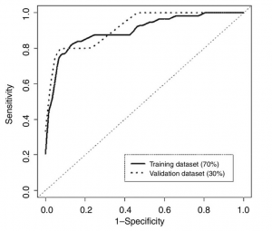
Here’s a graph showing how the error rate of the test changes with the numerical threshold used for diagnosis (figure 4, panel B, from the research paper)

pancreatic

As you move from left to right the threshold decreases; the test is more sensitive (picks up more of the true cases), but less specific (diagnoses more people who really don’t have cancer). The area under this curve is a simple summary of test accuracy, and that’s where the 90% number came from.  At what the researchers decided was the optimal threshold, the test correctly reported 82% of early-stage pancreatic cancers, but falsely reported a positive result in 11% of healthy subjects.  These figures are from the set of people whose data was used in putting the test together; in a new set of people (“validation dataset”) the error rate was very slightly worse.

The research was done with an approximately equal number of healthy people and people with early-stage pancreatic cancer. They did it that way because that gives the most information about the test for given number of people.  It’s reasonable to hope that the area under the curve, and the sensitivity and specificity of the test will be the same in the general population. Even so, the accuracy (in the non-technical meaning of the word) won’t be.

When you give this test to people in the general population, nearly all of them will not have pancreatic cancer. I don’t have NZ data, but in the UK the current annual rate of new cases goes from 4 people out of 100,000 at age 40 to 100 out of 100,000 people 85+.   The average over all ages is 13 cases per 100,000 people per year.

If 100,000 people are given the test and 13 have early-stage pancreatic cancer, about 10 or 11 of the 13 cases will have positive tests, but so will 11,000 healthy people.  Of those who test positive, 99.9% will not have pancreatic cancer.  This might still be useful, but it’s not what most people would think of as 90% accuracy.


April 10, 2015

Odds and probabilities

When quoting results of medical research there’s often confusion between odds and probabilities, but there are stories in the Herald and Stuff at the moment that illustrate the difference.

As you know (unless you’ve been on Mars with your eyes shut and your fingers in your ears), Jeremy Clarkson will no longer be presenting Top Gear, and the world is waiting with bated breath to hear about his successor.  Coral, a British firm of bookmakers, say that Sue Perkins is the current favourite.

The Herald quotes the Daily Mail, and so gives the odds as odds:

It has made her evens for the role, ahead of former X-factor presenter Dermot O’Leary who is 2-1 and British model Jodie Kidd who is third at 5-2.

Stuff translates these into NZ gambling terms, quoting the dividend, which is the reciprocal of the probability at which these would be regarded as fair bets

Bookmaker Coral have Perkins as the equivalent of a $2 favourite after a flurry of bets, while British-Irish presenter Dermot O’Leary was at $3 and television personality and fashion model Jodie Kidd at $3.50.

An odds of 5-2 means that betting £2 and winning gives you a profit of £5.  The NZ approach is to quote the total money you get back: a bet of $2 gets you $2 back plus $5 profit, for a total of $7, so a bet of $1 would get you $3.50.

The fair probability of winning for an odds of 5-2 is 2/(5+2); the fair probability for a dividend of $3.50 is 1/3.50, the same number.

Of course, if these were fair bets the bookies would go out of business: the actual implied probability for Jodie Kidd is lower than 1/3.5 and the actual implied probability for Sue Perkins is lower than 0.5.  On top of that, there is no guarantee the betting public is well calibrated on this issue.


February 27, 2015

Quake prediction: how good does it need to be?

From a detailed story in the ChCh Press, (via Eric Crampton) about various earthquake-prediction approaches

About 40 minutes before the quake began, the TEC in the ionosphere rose by about 8 per cent above expected levels. Somewhat perplexed, he looked back at the trend for other recent giant quakes, including the February 2010 magnitude 8.8 event in Chile and the December 2004 magnitude 9.1 quake in Sumatra. He found the same increase about the same time before the quakes occurred.

Heki says there has been considerable academic debate both supporting and opposing his research.

To have 40 minutes warning of a massive quake would be very useful indeed and could help save many lives. “So, why 40 minutes?” he says. “I just don’t know.”

He says if the link were to be proved more firmly in the future it could be a useful warning tool. However, there are drawbacks in that the correlation only appears to exist for the largest earthquakes, whereas big quakes of less than magnitude 8.0 are far more frequent and still cause death and devastation. Geomagnetic storms can also render the system impotent, with fluctuations in the total electron count masking any pre-quake signal.

Let’s suppose that with more research everything works out, and there is a rise in this TEC before all very large quakes. How much would this help in New Zealand? The obvious place is Wellington. A quake over 8.0 magnitude has been observed in the area in 1855, when it triggered a tsunami. A repeat would also shatter many of the earthquake-prone buildings. A 40-minute warning could save many lives. It appears that TEC shouldn’t be that expensive to measure: it’s based on observing the time delays in GPS satellite transmissions as they pass through the ionosphere, so it mostly needs a very accurate clock (in fact, NASA publishes TEC maps every five minutes). Also, it looks like it would be very hard to hack the ionosphere to force the alarm to go off. The real problem is accuracy.

The system will have false positives and false negatives. False negatives (missing a quake) aren’t too bad, since that’s where you are without the system. False positives are more of a problem. They come in two forms: when the alarm goes off completely in the absence of a quake, and when there is a quake but no tsunami or catastrophic damage.

Complete false predictions would need to be very rare. If you tell everyone to run for the hills and it turns out to be sunspots or the wrong kind of snow, they will not be happy: the cost in lost work (and theft?) would be substantial, and there would probably be injuries.  Partial false predictions, where there was a large quake but it was too far away or in the wrong direction to cause a tsunami, would be just as expensive but probably wouldn’t cause as much ill-feeling or skepticism about future warnings.

Now for the disappointment. The story says “there has been considerable academic debate”. There has. For example, in a (paywalled) paper from 2013 looking at the Japanese quake that prompted Heki’s idea

A detailed analysis of the ionospheric variability in the 3 days before the earthquake is then undertaken, where a simultaneous increase in foF2 and the Es layer peak plasma frequency, foEs, relative to the 30-day median was observed within 1 h before the earthquake. A statistical search for similar simultaneous foF2 and foEs increases in 6 years of data revealed that this feature has been observed on many other occasions without related seismic activity. Therefore, it is concluded that one cannot confidently use this type of ionospheric perturbation to predict an impending earthquake.

In translation: you need to look just right to see this anomaly, and there are often anomalies like this one without quakes. Over four years they saw 24 anomalies, only one shortly before a quake.  Six complete false positives per year is obviously too many.  Suppose future research could refine what the signal looks like and reduce the false positives by a factor of ten: that’s still evacuation alarms with no quake more than once every two years. I’m pretty sure that’s still too many.